Back propagation
This notebook is copied from Andrej Karpathy's Backpropagation lecture on youtube. I added a diagram and with the help of Claude, included some formulas in mathjax format.
from IPython.display import display, HTML
display(HTML("<style>.container { width:85% !important; }</style>"))
import torch
%matplotlib inline
import random
words = open('names.txt', 'r').read().splitlines()
print(len(words))
print(max(len(w) for w in words))
print(words[:8])
32033
15
['emma', 'olivia', 'ava', 'isabella', 'sophia', 'charlotte', 'mia', 'amelia']
# build the vocabulary of characters and mappings to/from integers
chars = sorted(list(set(''.join(words))))
stoi = {s: i + 1 for i, s in enumerate(chars)}
stoi['.'] = 0
itos = {i: s for s, i in stoi.items()}
vocab_size = len(itos)

print(stoi)
print(itos)
print(vocab_size)
{'a': 1, 'b': 2, 'c': 3, 'd': 4, 'e': 5, 'f': 6, 'g': 7, 'h': 8, 'i': 9, 'j': 10, 'k': 11, 'l': 12, 'm': 13, 'n': 14, 'o': 15, 'p': 16, 'q': 17, 'r': 18, 's': 19, 't': 20, 'u': 21, 'v': 22, 'w': 23, 'x': 24, 'y': 25, 'z': 26, '.': 0}
{1: 'a', 2: 'b', 3: 'c', 4: 'd', 5: 'e', 6: 'f', 7: 'g', 8: 'h', 9: 'i', 10: 'j', 11: 'k', 12: 'l', 13: 'm', 14: 'n', 15: 'o', 16: 'p', 17: 'q', 18: 'r', 19: 's', 20: 't', 21: 'u', 22: 'v', 23: 'w', 24: 'x', 25: 'y', 26: 'z', 0: '.'}
27
# build the dataset
block_size = 3  # context length: how many characters do we take to predict the next one?


def build_dataset(words):
    X, Y = [], []

    for w in words:
        context = [0] * block_size
        for ch in w + '.':
            ix = stoi[ch]
            X.append(context)
            Y.append(ix)
            context = context[1:] + [ix]  # crop and append

    X = torch.tensor(X)
    Y = torch.tensor(Y)
    print(X.shape, Y.shape)
    return X, Y
random.seed(42)
random.shuffle(words)
n1 = int(0.8 * len(words))
n2 = int(0.9 * len(words))

Xtr, Ytr = build_dataset(words[:n1])  # 80%
Xdev, Ydev = build_dataset(words[n1:n2])  # 10%
Xte, Yte = build_dataset(words[n2:])  # 10%
torch.Size([182625, 3]) torch.Size([182625])
torch.Size([22655, 3]) torch.Size([22655])
torch.Size([22866, 3]) torch.Size([22866])
Compare manual gradients with PyTorch gradients
# utility function we will use later when comparing manual
# gradients to PyTorch gradients
def cmp(s, dt, t):
  ex = torch.all(dt == t.grad).item()
  app = torch.allclose(dt, t.grad)
  maxdiff = (dt - t.grad).abs().max().item()

  print(f'{s:15s} | exact: {str(ex):5s} | approximate: {str(app):5s} | maxdiff: {maxdiff}')
Model
n_embd = 10  # the dimensionality of the character embedding vectors
n_hidden = 64  # the number of neurons in the hidden layer of the MLP

g = torch.Generator().manual_seed(2147483647)  # for reproducibility
C = torch.randn((vocab_size, n_embd), generator=g)

# Note: I am initializing many of these parameters in non-standard ways
# because sometimes initializing with e.g. all zeros could mask an incorrect
# implementation of the backward pass.

# Layer 1
W1 = torch.randn((n_embd * block_size, n_hidden), generator=g) * (5/3) / ((n_embd * block_size) ** 0.5)
b1 = torch.randn(n_hidden, generator=g) * 0.1  # using b1 just for fun, it's useless because of BN

# Layer 2
W2 = torch.randn((n_hidden, vocab_size), generator=g) * 0.1
b2 = torch.randn(vocab_size, generator=g) * 0.1

# BatchNorm parameters
bngain = torch.randn((1, n_hidden)) * 0.1 + 1.0
bnbias = torch.randn((1, n_hidden)) * 0.1

parameters = [C, W1, b1, W2, b2, bngain, bnbias]
print(sum(p.nelement() for p in parameters))  # number of parameters in total

for p in parameters:
    p.requires_grad = True
4137
-
you will note that I changed the initialization a little bit to be small numbers. so normally you would set the biases to be all zero, here I am setting them to be small random numbers
-
I'm doing this because if your variables are initialized to exactly zero, sometimes what can happen is that can mask an incorrect implementation of a gradient. Because when everything is zero, it sort of simplifies and gives you a much simpler expression of the gradient than you would otherwise get. so by making it small numbers, I'm trying to unmask those potential errors in these calculations.
-
You also notice that I'm using
b1in the first layer. I'm using a bias, despite batch normalization right afterwards so this would typically not be what you do because we talked about the fact that you don't need a bias, but I'm doing this here just for fun because we're going to have a gradient with respect to it and we can check that we are still calculating it correctly, even though this bias is spurious.
batch_size = 32
n = batch_size  # a shorter variable also, for convenience
# construct a minibatch
ix = torch.randint(0, Xtr.shape[0], (batch_size,), generator=g)
Xb, Yb = Xtr[ix], Ytr[ix]  # batch X,Y

# forward pass, "chunkated" into smaller steps that are possible to backward one at a time
emb = C[Xb] # embed the characters into vectors
embcat = emb.view(emb.shape[0], -1) # concatenate the vectors
# Linear layer 1
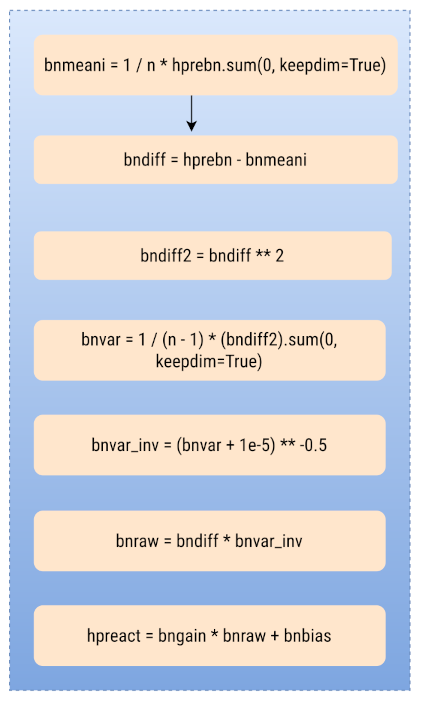
hprebn = embcat @ W1 + b1 # hidden layer pre-activation
# BatchNorm layer
bnmeani = 1 / n * hprebn.sum(0, keepdim=True)
bndiff = hprebn - bnmeani
bndiff2 = bndiff ** 2
bnvar = 1/(n - 1) * (bndiff2).sum(0, keepdim=True) # note: Bessel's correction (dividing by n-1, not n)
bnvar_inv = (bnvar + 1e-5) ** -0.5
bnraw = bndiff * bnvar_inv
hpreact = bngain * bnraw + bnbias
# Non-linearity
h = torch.tanh(hpreact) # hidden layer
# Linear layer 2
logits = h @ W2 + b2 # output layer
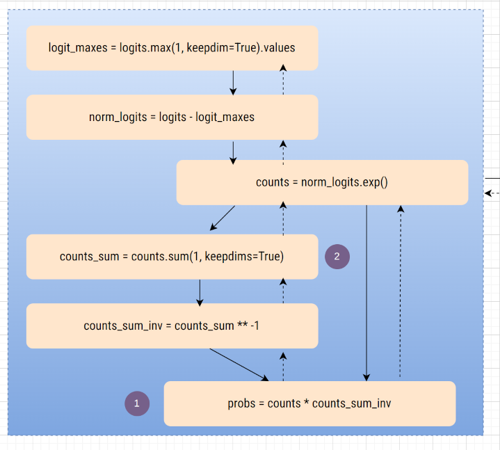
# cross entropy loss (same as F.cross_entropy(logits, Yb))
logit_maxes = logits.max(1, keepdim=True).values
norm_logits = logits - logit_maxes # subtract max for numerical stability
counts = norm_logits.exp()
counts_sum = counts.sum(1, keepdims=True)
counts_sum_inv = counts_sum ** -1 # if I use (1.0 / counts_sum) instead then I can't get backprop to be bit exact...
probs = counts * counts_sum_inv
logprobs = probs.log()
loss = -logprobs[range(n), Yb].mean()
# PyTorch backward pass
for p in parameters:
p.grad = None
for t in [logprobs, probs, counts, counts_sum, counts_sum_inv, # afaik there is no cleaner way
norm_logits, logit_maxes, logits, h, hpreact, bnraw,
bnvar_inv, bnvar, bndiff2, bndiff, hprebn, bnmeani,
embcat, emb]:
t.retain_grad()
loss.backward()
loss
tensor(3.3370, grad_fn=<NegBackward0>)
1. Calculate gradients manually
1.1 - dlogprobs
What is inside logprobs? the shape of this is
32x27. so it's not going to surprise you that
dlogprobs should also be an array of size 32x27
because we want the derivative loss with respect to all of its
elements. so the sizes of those are always going to be equal.
logprobs.shape
torch.Size([32, 27])
# Log probabilities for the first example
logprobs[0]
tensor([-2.6348, -2.4467, -3.9582, -3.0119, -4.0011, -2.5303, -3.6968, -3.2992,
        -4.0318, -3.4415, -3.2962, -3.2963, -3.1708, -3.5384, -3.3256, -4.2714,
        -4.7225, -3.9659, -4.2721, -2.8946, -3.0463, -3.8758, -3.6494, -2.6431,
        -2.8635, -3.6323, -3.7748], grad_fn=<SelectBackward0>)
# labels for this batch
Yb
tensor([ 8, 14, 15, 22,  0, 19,  9, 14,  5,  1, 20,  3,  8, 14, 12,  0, 11,  0,
        26,  9, 25,  0,  1,  1,  7, 18,  9,  3,  5,  9,  0, 18])
# loss = -logprobs[range(n), Yb].mean()
-
Now, how does
logprobsinfluence the loss? Loss is negativelogprobsindexed withrange(n), YBand then the mean of that. -
Now, just as a reminder,
Ybis just basically an array of all the correct indices. So what we're doing here is we're taking thelogprobsarray of size 32x27 and then we are going in every single row, and in each row we are plucking out the index 8 and then 14 and 15 and so on. -
So we're going down the rows That's the iterator range of
nand then we are always plucking out the index at the column specified by this tensorYb. So in the 0th row, we are taking the 8th column. In the first row, we're taking the 14th column, etc.
Calculating loss in Python
import torch.nn.functional as F

def get_loss():
    loss = 0

    for i in range(n):
        true_label_index = Yb[i].item()
        one_hot = (F.one_hot(torch.tensor(true_label_index), 27))
        one_hot_sum = 0

        for k in range(27):
            one_hot_sum += one_hot[k] * logprobs[i][k]

        loss += one_hot_sum

    print(f"Loss: {(-loss / n).item()}")

get_loss()
Loss: 3.3370251655578613
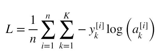
Cross entropy loss
n- batch sizeK- number of classesi- index of the sample in the batchk- index of the classL- loss
is the true label (0 or 1) for the i-th example and k-th class. This assumes one hot encoding. is the predicted probability for the i-th example and k-th class
Derivative of mean
From this matrix, we're picking a single entry for each example and taking mean of them.
# Derivative of "mean".
# sample
# l = -(a + b + c) / 3
# l = -a/3 -b/3 - c/3
# dl/da = -1/3
# dl/db = -1/3
# dl/dc = -1/3
You see that logprobs shape is 32x27. But only 32
of them participate in the loss calculation. So what's the
derivative of all the other, most of the elements that do not
get plucked out here? Well,
their gradient intuitively is zero. And that's
because they did not participate in the loss.
So most of these numbers inside this tensor does not feed into the loss and so if we were to change these numbers, then the loss doesn't change, which is the equivalent of way of saying that the derivative with respect to them is zero. They don't impact it.
dlogprobs = torch.zeros_like(logprobs)
dlogprobs[range(n), Yb] = -1.0 / n

cmp("logprobs", dlogprobs, logprobs)
logprobs | exact: True | approximate: True | maxdiff: 0.0
1.2 - dprobs
# logprobs = probs.log()
dprobs = (1.0 / probs) * dlogprobs

cmp("probs", dprobs, probs)
probs | exact: True | approximate: True | maxdiff: 0.0
-
So if
probesis very, very close to 1, that means your network is currently predicting the character correctly, then1/probswill become 1 over 1, anddlogprobsjust gets pass-through. -
But if probabilities are incorrectly assigned, so if the
correct character here is getting a very low probability, then
1.0 / probswill be higher and then multiplied bydlogprobs - So basically what this line is doing intuitively is taking to the examples that have a very low probability currently assigned and it's boosting their gradient.
1.3 - dcounts_sum_inv
# probs = counts * counts_sum_inv
probs.shape, counts.shape, counts_sum_inv.shape
(torch.Size([32, 27]), torch.Size([32, 27]), torch.Size([32, 1]))
probs = counts * counts_sum_inv
countsis 32 x 27counts_sum_invis 32 x 1
This operation is composed of two steps:
-
A Broadcast occurs (Each row of
counts_sum_invis replicated 27 times along the column - virtually making a 32 x 27 matrix) - Element wise multiplication occurs
counts.shape, counts_sum_inv.shape
(torch.Size([32, 27]), torch.Size([32, 1]))
(counts * counts_sum_inv).shape
torch.Size([32, 27])
# NOTE: If a broadcast occurs during forward prop,
#       a sum() operation will be performed during backprop.
dcounts_sum_inv = (counts * dprobs).sum(axis=1, keepdim=True)
cmp("counts_sum_inv", dcounts_sum_inv, counts_sum_inv)
counts_sum_inv | exact: True | approximate: True | maxdiff: 0.0
counts_sum_inv.shape == dcounts_sum_inv.shape
True
1.4 - dcounts - [1]
-
countsis used to evaluate two valuesprobscounts_sum
-
so, when finding
dcounts, these two expressions need to be considered.
dprobs.shape
torch.Size([32, 27])
# 32, 1
# 32, 27
# => 32, 27
dcounts = counts_sum_inv * dprobs
1.5 - counts_sum
# counts_sum_inv = counts_sum ** -1
dcounts_sum = (-counts_sum ** -2) * dcounts_sum_inv

cmp("counts_sum", dcounts_sum, counts_sum)
counts_sum | exact: True | approximate: True | maxdiff: 0.0
1.6 - dcounts [2]
- This derivative is a 32x27 matrix filled with ones.
- Each element in this matrix represents the partial derivative of the sum with respect to the corresponding element in the original matrix A. The derivative is 1 for each element because changing any element in A by a small amount δ will change the corresponding row sum by exactly δ.
counts.shape, counts_sum.shape
(torch.Size([32, 27]), torch.Size([32, 1]))
# counts_sum = counts.sum(1, keepdims=True)
dcounts += torch.ones_like(counts) * dcounts_sum
cmp("counts", dcounts, counts)
counts | exact: True | approximate: True | maxdiff: 0.0
1.7 - dnorm_logits
# counts = norm_logits.exp()
dnorm_logits = counts * dcounts
cmp("norm_logits", dnorm_logits, norm_logits)
norm_logits | exact: True | approximate: True | maxdiff: 0.0
1.8 - dlogits - [1]
# norm_logits = logits - logit_maxes
# Implicit bradcasting is happening here.
logits.shape, logit_maxes.shape
(torch.Size([32, 27]), torch.Size([32, 1]))
Derivatives
dlogits = torch.ones_like(logits) * dnorm_logits
1.9 - dlogit_maxes
dlogit_maxes = (-torch.ones_like(logits) * dnorm_logits).sum(axis=1, keepdim=True)
cmp("dlogit_maxes", dlogit_maxes, logit_maxes)
dlogit_maxes | exact: True | approximate: True | maxdiff: 0.0
# Set the print options to show 4 decimal places
torch.set_printoptions(precision=8, sci_mode=False)
print(dlogit_maxes)
tensor([[    -0.00000000],
        [     0.00000000],
        [    -0.00000000],
        [    -0.00000000],
        [     0.00000000],
        [     0.00000000],
        [    -0.00000000],
        [    -0.00000000],
        [     0.00000000],
        [    -0.00000001],
        [    -0.00000000],
        [     0.00000000],
        [    -0.00000000],
        [     0.00000001],
        [     0.00000000],
        [    -0.00000000],
        [     0.00000000],
        [     0.00000001],
        [    -0.00000000],
        [     0.00000000],
        [    -0.00000000],
        [    -0.00000000],
        [    -0.00000000],
        [     0.00000001],
        [    -0.00000000],
        [     0.00000000],
        [     0.00000000],
        [     0.00000000],
        [     0.00000000],
        [    -0.00000000],
        [     0.00000001],
        [     0.00000000]], grad_fn=<SumBackward1>)
NOTE:
logit_maxes = logits.max(1, keepdim=True).values
norm_logits = logits - logit_maxes  # subtract max for numerical stability
counts = norm_logits.exp()
We've talked previously in the
previous lecture
that the only reason we're doing this is for the numerical
stability of the soft max that we are implementing here and we
talked about how if you take these logits for any one of these
examples so one row of this logits tensor if you add or subtract
any value equally to all the elements then the value of the
probs will be unchanged. you're not changing the soft max! the
only thing that this is doing is it's making sure that
exp() doesn't overflow and the reason we're using a
max() is because then we are guaranteed that each
row of logits, the highest number is zero. And so this will be
safe.
And so basically that has repercussions. If it is the case that
changing logit_maxes does not change the probs and
therefore there's not change the loss, then the gradient on
logit_maxes should be zero, right? Because saying
those two things is the same. So indeed, we hope that this is
very, very small numbers. Indeed, we hope this is zero. Now,
because of floating point sort of wonkiness, this doesn't come
out exactly zero, only in some of the rows it does. But we get
extremely small values, like 1e -9 or -10.
And so this is telling us that the values of
logit_maxes are not impacting the loss as they
shouldn't. It feels kind of weird to back propagate through this
branch, honestly, because if you have any implementation of like
F.cross_entropy() and PyTorch, and you block
together all these elements and you're not doing the back
propagation piece by piece, then you would probably assume that
the derivative through here is exactly zero.
So you would be sort of skipping this branch because it's only done for numerical stability. But it's interesting to see that even if you break up everything into the full atoms and you still do the computation as you'd like with respect to numerical stability, the correct thing happens and you still get a very, very small gradients here, basically reflecting the fact that the values of these do not matter with respect to the final loss.
1.10 - dlogits - [2]
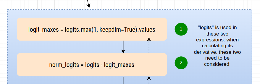
logits.shape
torch.Size([32, 27])
Forward operation
# For each row, identify the max value.
logit_maxes = logits.max(1, keepdim=True).values
Derivative
- Each row of the derivative matrix will have exactly one 1 and twenty-six 0s.
-
The position of the 1 in each row corresponds to the position
of the maximum value in that row of the original
logitsmatrix.
dlogits += F.one_hot(logits.max(1).indices, num_classes=logits.shape[1]) * dlogit_maxes

# verify
cmp("dlogits", dlogits, logits)
dlogits | exact: True | approximate: True | maxdiff: 0.0
1.11 - dh, dw2, db2
dlogits.shape, h.shape, W2.shape, b2.shape
(torch.Size([32, 27]),
 torch.Size([32, 64]),
 torch.Size([64, 27]),
 torch.Size([27]))
# Linear layer 2
logits = h @ W2 + b2  # output layer
- The simplified equation:
- The expanded matrix form:
- The resulting individual equations:
Derivatives
- The equations represent partial derivatives of L with respect to different elements of matrix a:
-
dL/dd11is the global derivative (for chian rule) -
It is multiplied with local derivative of
a11, which isb11 -
Since
a11is used twice in this multiplication, its derivatives should be summed.
- These equations are then represented in matrix form:
- This is then shown to be equivalent to:
- Finally, this is expressed in a more compact form using matrix notation:
Here, @ represents matrix multiplication, and is the transpose of matrix b.
This set of equations appears to be demonstrating the chain rule for matrix derivatives, specifically how the gradient of L with respect to a is related to the gradient with respect to d and the elements of matrix b.
Similarly
# logits = h @ W2 + b2
dh = dlogits @ W2.T
dW2 = h.T @ dlogits
db2 = dlogits.sum(axis=0)
# verify
cmp("dh", dh, h)
cmp("dW2", dW2, W2)
cmp("db2", db2, b2)
dh              | exact: True  | approximate: True  | maxdiff: 0.0
dW2             | exact: True  | approximate: True  | maxdiff: 0.0
db2             | exact: True  | approximate: True  | maxdiff: 0.0
1.12 - dhpreact
# h = torch.tanh(hpreact)

dhpreact = (1.0 - h**2) * dh
cmp("hpreact", dhpreact, hpreact)
hpreact | exact: False | approximate: True | maxdiff: 4.656612873077393e-10
Batch normalization
1.13 - dbngain, dbnraw, dbnbias
# hpreact = bngain * bnraw + bnbias
hpreact.shape, bngain.shape, bnraw.shape, bnbias.shape
(torch.Size([32, 64]),
 torch.Size([1, 64]),
 torch.Size([32, 64]),
 torch.Size([1, 64]))
# During forward prop,
#   bngain -> 1, 64
#   bnraw ->  32, 64
# When they're mulitplied, "bngain" is broadcast to become "32, 64" (1 row => 32 rows)
# so, During backprop, we need to sum() the gradients in 0th dim.
dbngain = (bnraw * dhpreact).sum(0, keepdim=True)

dbnraw = (bngain * dhpreact)
dbnbias = dhpreact.sum(0, keepdim=True)

cmp("bngain", dbngain, bngain)
cmp("bnraw", dbnraw, bnraw)
cmp("bnbias", dbnbias, bnbias)
bngain          | exact: False | approximate: True  | maxdiff: 1.862645149230957e-09
bnraw           | exact: False | approximate: True  | maxdiff: 4.656612873077393e-10
bnbias          | exact: False | approximate: True  | maxdiff: 3.725290298461914e-09
1.14 - dbndiff [1]
# bnraw = bndiff * bnvar_inv
dbnraw.shape, bnraw.shape, bndiff.shape, bnvar_inv.shape
(torch.Size([32, 64]),
 torch.Size([32, 64]),
 torch.Size([32, 64]),
 torch.Size([1, 64]))
dbndiff = (bnvar_inv * dbnraw)
1.15 - dbnvar_inv
dbnvar_inv = (bndiff * dbnraw).sum(0, keepdim=True)
bnvar_inv.shape, dbnvar_inv.shape
(torch.Size([1, 64]), torch.Size([1, 64]))
cmp("bnvar_inv", dbnvar_inv, bnvar_inv)
bnvar_inv | exact: False | approximate: True | maxdiff: 3.725290298461914e-09
1.16 - dbnvar
# bnvar_inv = (bnvar + 1e-5) ** -0.5
dbnvar = (-0.5 * ((bnvar + 1e-5) ** -1.5)) * dbnvar_inv

cmp("dbnvar", dbnvar, bnvar)
dbnvar | exact: False | approximate: True | maxdiff: 8.149072527885437e-10
1.17 - dbndiff2
# bnvar = 1 / (n - 1) * (bndiff2).sum(0, keepdim=True) # note: Bessel's correction (dividing by n-1, not n)
Bessel's correction
It turns out that there are two ways of estimating variance of an array.
- One is the biased estimate, which is
1/n -
And the other one is the unbiased estimate, which is
1/n-1
bnvar.shape, bndiff2.shape
(torch.Size([1, 64]), torch.Size([32, 64]))
dbndiff2 = (1.0 / (n-1)) * torch.ones_like(bndiff2) * dbnvar

cmp("bndiff2", dbndiff2, bndiff2)
bndiff2 | exact: False | approximate: True | maxdiff: 2.546585164964199e-11
1.18 - dbndiff [2]
# bndiff2 = bndiff ** 2
dbndiff += (2 * bndiff) * (dbndiff2)

cmp("bndiff", dbndiff, bndiff)
bndiff | exact: False | approximate: True | maxdiff: 4.656612873077393e-10
1.19 - dbnmeani
# bndiff = hprebn - bnmeani
bndiff.shape, hprebn.shape, bnmeani.shape
(torch.Size([32, 64]), torch.Size([32, 64]), torch.Size([1, 64]))
dbnmeani = (-torch.ones_like(bndiff) * dbndiff).sum(0)
cmp("bnmeani", dbnmeani, bnmeani)
bnmeani | exact: False | approximate: True | maxdiff: 3.725290298461914e-09
1.20 - dhprebn [1]
# bndiff = hprebn - bnmeani
dhprebn = dbndiff.clone()
1.21 - dhprebn - [2]
# bnmeani = 1 / n * hprebn.sum(0, keepdim=True)
dhprebn += 1.0/n * (torch.ones_like(hprebn) * dbnmeani)

cmp("hprebn", dhprebn, hprebn)
hprebn | exact: False | approximate: True | maxdiff: 4.656612873077393e-10
1.22 - dembcat, dW1, db1
# hprebn = embcat @ W1 + b1
hprebn.shape, embcat.shape, W1.shape, b1.shape
(torch.Size([32, 64]),
 torch.Size([32, 30]),
 torch.Size([30, 64]),
 torch.Size([64]))
is of the form:
Here, @ represents matrix multiplication, and is the transpose of matrix b.
This set of equations appears to be demonstrating the chain rule for matrix derivatives, specifically how the gradient of L with respect to a is related to the gradient with respect to d and the elements of matrix b.
Similarly
dembcat = dhprebn @ W1.T
dW1 = embcat.T @ dhprebn
db1 = dhprebn.sum(0)
cmp("embcat", dembcat, embcat)
cmp("W2", dW2, W2)
cmp("b2", db2, b2)
embcat          | exact: False | approximate: True  | maxdiff: 1.3969838619232178e-09
W2              | exact: True  | approximate: True  | maxdiff: 0.0
b2              | exact: True  | approximate: True  | maxdiff: 0.0
1.23 - demb
# embcat = emb.view(emb.shape[0], -1)
embcat.shape, emb.shape
(torch.Size([32, 30]), torch.Size([32, 3, 10]))
demb = dembcat.view(emb.shape)

cmp("emb", demb, emb)
emb | exact: False | approximate: True | maxdiff: 1.3969838619232178e-09
1.24 - dC
# emb = C[Xb]
emb.shape, C.shape, Xb.shape
(torch.Size([32, 3, 10]), torch.Size([27, 10]), torch.Size([32, 3]))
dC = torch.zeros_like(C)

for k in range(Xb.shape[0]):
    for j in range(Xb.shape[1]):
        ix = Xb[k,j]
        dC[ix] += demb[k,j]
cmp("logprobs", dlogprobs, logprobs)
cmp("probs", dprobs, probs)
cmp("counts_sum_inv", dcounts_sum_inv, counts_sum_inv)
cmp("counts_sum", dcounts_sum, counts_sum)
cmp("counts", dcounts, counts)
cmp("norm_logits", dnorm_logits, norm_logits)
cmp("logit_maxes", dlogit_maxes, logit_maxes)
cmp("logits", dlogits, logits)
cmp("h", dh, h)
cmp("W2", dW2, W2)
cmp("b2", db2, b2)
cmp("hpreact", dhpreact, hpreact)
cmp("bngain", dbngain, bngain)
cmp("bnraw", dbnraw, bnraw)
cmp("bnbias", dbnbias, bnbias)
cmp("bnvar_inv", dbnvar_inv, bnvar_inv)
cmp("dbnvar", dbnvar, bnvar)
cmp("bndiff2", dbndiff2, bndiff2)
cmp("bndiff", dbndiff, bndiff)
cmp("bnmeani", dbnmeani, bnmeani)
cmp("hprebn", dhprebn, hprebn)
cmp("embcat", dembcat, embcat)
cmp("W2", dW2, W2)
cmp("b2", db2, b2)
cmp("emb", demb, emb)
cmp("C", dC, C)
logprobs        | exact: True  | approximate: True  | maxdiff: 0.0
probs           | exact: True  | approximate: True  | maxdiff: 0.0
counts_sum_inv  | exact: True  | approximate: True  | maxdiff: 0.0
counts_sum      | exact: True  | approximate: True  | maxdiff: 0.0
counts          | exact: True  | approximate: True  | maxdiff: 0.0
norm_logits     | exact: True  | approximate: True  | maxdiff: 0.0
logit_maxes     | exact: True  | approximate: True  | maxdiff: 0.0
logits          | exact: True  | approximate: True  | maxdiff: 0.0
h               | exact: True  | approximate: True  | maxdiff: 0.0
W2              | exact: True  | approximate: True  | maxdiff: 0.0
b2              | exact: True  | approximate: True  | maxdiff: 0.0
hpreact         | exact: False | approximate: True  | maxdiff: 4.656612873077393e-10
bngain          | exact: False | approximate: True  | maxdiff: 1.862645149230957e-09
bnraw           | exact: False | approximate: True  | maxdiff: 4.656612873077393e-10
bnbias          | exact: False | approximate: True  | maxdiff: 3.725290298461914e-09
bnvar_inv       | exact: False | approximate: True  | maxdiff: 3.725290298461914e-09
dbnvar          | exact: False | approximate: True  | maxdiff: 8.149072527885437e-10
bndiff2         | exact: False | approximate: True  | maxdiff: 2.546585164964199e-11
bndiff          | exact: False | approximate: True  | maxdiff: 4.656612873077393e-10
bnmeani         | exact: False | approximate: True  | maxdiff: 3.725290298461914e-09
hprebn          | exact: False | approximate: True  | maxdiff: 4.656612873077393e-10
embcat          | exact: False | approximate: True  | maxdiff: 1.3969838619232178e-09
W2              | exact: True  | approximate: True  | maxdiff: 0.0
b2              | exact: True  | approximate: True  | maxdiff: 0.0
emb             | exact: False | approximate: True  | maxdiff: 1.3969838619232178e-09
C               | exact: False | approximate: True  | maxdiff: 7.450580596923828e-09
2. Derivatives of Softmax and Cross-Entropy Loss
# Linear layer 2
logits = h @ W2 + b2  # output layer
# cross entropy loss (same as F.cross_entropy(logits, Yb))
logit_maxes = logits.max(1, keepdim=True).values
norm_logits = logits - logit_maxes  # subtract max for numerical stability
counts = norm_logits.exp()
counts_sum = counts.sum(1, keepdims=True)
counts_sum_inv = counts_sum ** -1  # if I use (1.0 / counts_sum) instead then I can't get backprop to be bit exact...
probs = counts * counts_sum_inv
logprobs = probs.log()

loss = -logprobs[range(n), Yb].mean()
Rather than implementing Softmax, and Loss functions, we can use PyTorch's built-in functions to calculate the loss.
loss_fast = F.cross_entropy(logits, Yb)
print(loss_fast.item(), 'diff:', (loss_fast - loss).item())
3.337024688720703 diff: -2.384185791015625e-07
Backward pass
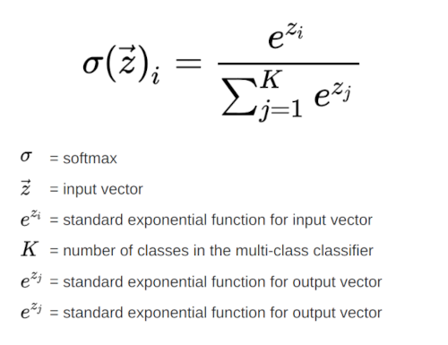
Softmax function:
- This converts logits to probabilities.
Cross-entropy loss:
- Where y is the index of the correct class.
Gradient of loss with respect to logits:
For i ≠ y (incorrect class):
For i = y (correct class):
Derivation for i ≠ y:
Derivation for i = y:
These derivations show that the gradient with respect to each logit is simply the difference between the predicted probability and the true probability (which is 0 for incorrect classes and 1 for the correct class).
dlogits = F.softmax(logits, 1)
dlogits[range(n), Yb] -= 1
dlogits /= n

cmp('logits', dlogits, logits)
logits | exact: False | approximate: True | maxdiff: 7.450580596923828e-09
import matplotlib.pyplot as plt

plt.figure(figsize=(8, 8))
plt.imshow(dlogits.detach(), cmap='Blues')
<matplotlib.image.AxesImage at 0x75ed8c67b750>

3. backprop through batchnorm but all in one go
To complete this challenge look at the mathematical expression of the output of batchnorm, take the derivative w.r.t. its input, simplify the expression, and just write it out.
Forward pass
# Linear layer 1
hprebn = embcat @ W1 + b1  # hidden layer pre-activation
# BatchNorm layer
bnmeani = 1 / n * hprebn.sum(0, keepdim=True)
bndiff = hprebn - bnmeani
bndiff2 = bndiff ** 2
bnvar = 1/(n - 1) * (bndiff2).sum(0, keepdim=True)  # note: Bessel's correction (dividing by n-1, not n)
bnvar_inv = (bnvar + 1e-5) ** -0.5
bnraw = bndiff * bnvar_inv
hpreact = bngain * bnraw + bnbias
# Non-linearity
h = torch.tanh(hpreact)  # hidden layer
hpreact_fast = bngain * (hprebn - hprebn.mean(0, keepdim=True)) / torch.sqrt(hprebn.var(0, keepdim=True, unbiased=True) + 1e-5) + bnbias
print('max diff:', (hpreact_fast - hpreact).abs().max())
max diff: tensor( 0.00000048, grad_fn=<MaxBackward1>)
Backward pass
4. Using custom backprop
# Exercise 4: putting it all together!
# Train the MLP neural net with your own backward pass

# init
n_embd = 10 # the dimensionality of the character embedding vectors
n_hidden = 200 # the number of neurons in the hidden layer of the MLP

g = torch.Generator().manual_seed(2147483647) # for reproducibility
C  = torch.randn((vocab_size, n_embd),            generator=g)

# Layer 1
W1 = torch.randn((n_embd * block_size, n_hidden), generator=g) * (5/3)/((n_embd * block_size)**0.5)
b1 = torch.randn(n_hidden,                        generator=g) * 0.1

# Layer 2
W2 = torch.randn((n_hidden, vocab_size),          generator=g) * 0.1
b2 = torch.randn(vocab_size,                      generator=g) * 0.1

# BatchNorm parameters
bngain = torch.randn((1, n_hidden))*0.1 + 1.0
bnbias = torch.randn((1, n_hidden))*0.1

parameters = [C, W1, b1, W2, b2, bngain, bnbias]
print(sum(p.nelement() for p in parameters)) # number of parameters in total
for p in parameters:
  p.requires_grad = True

# same optimization as last time
max_steps = 200000
batch_size = 32
n = batch_size # convenience
lossi = []

# use this context manager for efficiency once your backward pass is written (TODO)
with torch.no_grad():

  # kick off optimization
  for i in range(max_steps):

    # minibatch construct
    ix = torch.randint(0, Xtr.shape[0], (batch_size,), generator=g)
    Xb, Yb = Xtr[ix], Ytr[ix] # batch X,Y

    # forward pass
    emb = C[Xb] # embed the characters into vectors
    embcat = emb.view(emb.shape[0], -1) # concatenate the vectors

    # Linear layer
    hprebn = embcat @ W1 + b1 # hidden layer pre-activation

    # BatchNorm layer
    # -------------------------------------------------------------
    bnmean = hprebn.mean(0, keepdim=True)
    bnvar = hprebn.var(0, keepdim=True, unbiased=True)
    bnvar_inv = (bnvar + 1e-5)**-0.5
    bnraw = (hprebn - bnmean) * bnvar_inv
    hpreact = bngain * bnraw + bnbias

    # -------------------------------------------------------------
    # Non-linearity
    h = torch.tanh(hpreact) # hidden layer

    logits = h @ W2 + b2 # output layer
    loss = F.cross_entropy(logits, Yb) # loss function

    # backward pass
    for p in parameters:
      p.grad = None

    #loss.backward() # use this for correctness comparisons, delete it later!

    # manual backprop! #swole_doge_meme
    # -----------------
    dlogits = F.softmax(logits, 1)
    dlogits[range(n), Yb] -= 1
    dlogits /= n

    # 2nd layer backprop
    dh = dlogits @ W2.T
    dW2 = h.T @ dlogits
    db2 = dlogits.sum(0)

    # tanh
    dhpreact = (1.0 - h**2) * dh

    # batchnorm backprop
    dbngain = (bnraw * dhpreact).sum(0, keepdim=True)
    dbnbias = dhpreact.sum(0, keepdim=True)
    dhprebn = bngain*bnvar_inv/n * (n*dhpreact - dhpreact.sum(0) - n/(n-1)*bnraw*(dhpreact*bnraw).sum(0))

    # 1st layer
    dembcat = dhprebn @ W1.T
    dW1 = embcat.T @ dhprebn
    db1 = dhprebn.sum(0)

    # embedding
    demb = dembcat.view(emb.shape)
    dC = torch.zeros_like(C)
    for k in range(Xb.shape[0]):
      for j in range(Xb.shape[1]):
        ix = Xb[k,j]
        dC[ix] += demb[k,j]

    grads = [dC, dW1, db1, dW2, db2, dbngain, dbnbias]
    # -----------------

    # update
    lr = 0.1 if i < 100000 else 0.01 # step learning rate decay
    for p, grad in zip(parameters, grads):
      #p.data += -lr * p.grad # old way of cheems doge (using PyTorch grad from .backward())
      p.data += -lr * grad # new way of swole doge TODO: enable

    # track stats
    if i % 10000 == 0: # print every once in a while
      print(f'{i:7d}/{max_steps:7d}: {loss.item():.4f}')
    lossi.append(loss.log10().item())

  #   if i >= 100: # TODO: delete early breaking when you're ready to train the full net
  #     break
12297
      0/ 200000: 3.8202
  10000/ 200000: 2.1700
  20000/ 200000: 2.3754
  30000/ 200000: 2.4753
  40000/ 200000: 2.0044
  50000/ 200000: 2.3516
  60000/ 200000: 2.4647
  70000/ 200000: 2.0118
  80000/ 200000: 2.3101
  90000/ 200000: 2.1598
 100000/ 200000: 1.9379
 110000/ 200000: 2.3239
 120000/ 200000: 1.9858
 130000/ 200000: 2.5301
 140000/ 200000: 2.3005
 150000/ 200000: 2.2094
 160000/ 200000: 1.9649
 170000/ 200000: 1.8325
 180000/ 200000: 1.9479
 190000/ 200000: 1.9015
# calibrate the batch norm at the end of training

with torch.no_grad():
  # pass the training set through
  emb = C[Xtr]
  embcat = emb.view(emb.shape[0], -1)
  hpreact = embcat @ W1 + b1
  # measure the mean/std over the entire training set
  bnmean = hpreact.mean(0, keepdim=True)
  bnvar = hpreact.var(0, keepdim=True, unbiased=True)
# evaluate train and val loss

@torch.no_grad() # this decorator disables gradient tracking
def split_loss(split):
  x,y = {
    'train': (Xtr, Ytr),
    'val': (Xdev, Ydev),
    'test': (Xte, Yte),
  }[split]

  emb = C[x] # (N, block_size, n_embd)
  embcat = emb.view(emb.shape[0], -1) # concat into (N, block_size * n_embd)
  hpreact = embcat @ W1 + b1
  hpreact = bngain * (hpreact - bnmean) * (bnvar + 1e-5)**-0.5 + bnbias
  h = torch.tanh(hpreact) # (N, n_hidden)
  logits = h @ W2 + b2 # (N, vocab_size)
  loss = F.cross_entropy(logits, y)
  print(split, loss.item())

split_loss('train')
split_loss('val')
train 2.0702784061431885
val 2.1081807613372803
# sample from the model
g = torch.Generator().manual_seed(2147483647 + 10)

for _ in range(20):

    out = []
    context = [0] * block_size # initialize with all ...
    while True:
      # ------------
      # forward pass:
      # Embedding
      emb = C[torch.tensor([context])] # (1,block_size,d)
      embcat = emb.view(emb.shape[0], -1) # concat into (N, block_size * n_embd)
      hpreact = embcat @ W1 + b1
      hpreact = bngain * (hpreact - bnmean) * (bnvar + 1e-5)**-0.5 + bnbias
      h = torch.tanh(hpreact) # (N, n_hidden)
      logits = h @ W2 + b2 # (N, vocab_size)
      # ------------
      # Sample
      probs = F.softmax(logits, dim=1)
      ix = torch.multinomial(probs, num_samples=1, generator=g).item()
      context = context[1:] + [ix]
      out.append(ix)
      if ix == 0:
        break

    print(''.join(itos[i] for i in out))
mona.
mayah.
see.
mad.
ryla.
renverlendraegustered.
elin.
shi.
jenleigh.
sanana.
sephanvitte.
mayshubergihira.
sten.
joselle.
joseulan.
brence.
ryyah.
fael.
yuva.
myshaydenhil.